Written By KYLE MATHIAS | AUDIO BASICS, MIXING
Digital audio has revolutionized the way we produce music – the noise floor is so low that we can basically ignore it, there’s more headroom than we could ever possibly need, and it exhibits totally linear, distortion-free behavior. Compared to analog, digital audio is higher-fidelity in every way imaginable.
But if this is the case, then why do so many engineers and producers today still use analog gear? And why do companies like Universal Audio (the sponsor of this post) continue to produce analog gear like the 1176 and the LA-2A as well as plugin emulations of analog consoles, compressors, and tape machines?

Higher-Fidelity vs Better
If we’re going to answer this question, it’s important that we first agree that there is a difference between “higher-fidelity” and “better”.
Fidelity means “the degree of exactness with which something is copied or reproduced”, while better… means “better”.
This is important because the secret behind analog audio being “better” in some cases can mostly be boiled down to the fact that it is not as “high-fidelity” as digital audio.
Digital audio is perfect. If you want a low-noise, clean, and distortion-free recording that faithfully represents the input signal being recorded, digital is the way to go.
Before digital audio was widely used in studios, the primary goal of most recording engineers was to make clean recordings with minimal noise and minimal distortion. But realizing this goal with analog gear came with a few challenges. For instance, take the behavior of an analog tape machine. If levels were set too low, the signal would be buried within the noise floor. If levels were set too high, the signal would be distorted.

Digital allowed engineers to realize the goal of a clean recording to a level that was simply unimaginable with analog tape. But when they finally had access to such a perfect tool, many of them realized that greater fidelity didn’t necessarily correlate to better sound.
Throughout the decades of producing music with analog equipment, engineers and listeners had developed a familiarity (and even an emotional connection) with the imperfections of analog gear. The sound of music itself had become intertwined with the idiosyncrasies of analog equipment.
So when digital audio removed all of those imperfections, the music was left sounding sterile and lifeless. And audio engineers quickly learned that while it’s easy to end up with too much distortion using analog, it’s just as easy to end up with too little distortion using digital. And that’s the main reason why we spend so much time and energy today trying to put that distortion, or analog magic, back into our digital productions.
Let’s discuss what happens when you pass a signal through analog gear and try to figure out what makes analog “analog”.
Harmonic Distortion
A typical digital audio system is perfectly linear for all practical purposes. That means a change to the input level will result in a proportional change to the output level. Take for example this signal chain…
An input signal, a linear EQ plugin, and an output signal.
With the EQ on this UA Precision Channel Strip, the input signal level doesn’t matter. Increasing the input signal level by 12 dB will just result in an equal increase to the output signal level. Regardless of the input level going into this EQ plugin, the EQ cut applied to the signal will remain the same.
This is true all the way up to the point where the input or output level exceeds 0 dB Full Scale, at which point the signal will be clipped in a fixed point digital audio system. But so long as we stay below 0 dB, the behavior is linear. In fact, many modern DAWs operate internally with floating point, which means they will maintain linearity even far beyond 0 dB FS.

One of the signature characteristics of analog gear is that it has a non-linear response to input levels. Typically, analog gear is designed for a linear response at its intended operating level but no analog circuit has unlimited headroom. And at a certain point, boosting the input signal by 12 dB will result in very audible distortion.
As you can hear in the video, overloading the input of a tape machine or saturating magnetic tape while recording wasn’t always a bad thing, even though it ultimately resulted in signal distortion. Those analog distortions actually brought character to the sound in many cases.
On the other hand, overloading the input of a digital system will almost always sound terrible because it results in digital clipping that very closely resembles a square wave. You’ve undoubtedly heard this when your mic input level exceeds 0 dB in your DAW during a recording session.

But, what is actually happening to the signal when the limits of each system are approached and exceeded?
First, by sending a 100 Hz sine wave out of an audio interface and back into the input there is a spike of energy at 100 Hz, that can be seen on a frequency analyzer, but nowhere else. This is true all the way up to 0 dBFS. If the signal level exceeds 0 dBFS by even .01 dB, we start to see some significant harmonic distortion.
All the way up to that point, the level of the sine wave just increases. But at the point where the signal actually exceeds that limit, there are a few additional frequencies that arise – and these are called harmonics.

The same is true the other way around. If we were to send a clean 100 Hz sine wave out of an interface, never exceeding 0 dB FS on the output, but increasing the preamp gain to the point where the signal level begins to exceed 0 dB FS on the input, we see some significant harmonics pop up at that exact moment. And as that signal is driven further into clipping, more harmonics are created and the level of those harmonics increases relative to the fundamental frequency.
We’ll see a similar outcome when we send a signal through a tape machine (or in this case, an emulation of a tape machine). But instead of getting a clean sound until we hit the absolute limit, we start seeing harmonics even before that point. And the relative levels of each harmonic frequency are a bit different, too.
These harmonics don’t just pop up in the electrical domain either. They can also arise naturally in acoustics. For example, playing a note A on the electric guitar with a fundamental frequency at 220 Hz won’t merely result in energy at the fundamental but will also excite some harmonic frequencies.
In all three of these cases – digital clipping, analog tape saturation, and playing a note on an acoustic instrument – the harmonics that arise follow a similar pattern. The harmonic series is found by adding the fundamental frequency to itself again and again.
In our initial examples, 100 Hz was the fundamental frequency, the second harmonic was 200 Hz, the third harmonic was 300 Hz, the fourth harmonic was 400 Hz, and so on.

Generally speaking, even order harmonics tend to sound sweeter to our ears compared to odd order harmonics. However, they can certainly both sound great in a mix. What’s more important is the relative blend of each harmonic frequency within this series and that’s a big part of the richness that gives each instrument (or electrical circuit) its own unique character.
Analog harmonic distortion tends to follow a pattern that more closely resembles the harmonic frequencies that unfold from a musical instrument. Hence, this type of harmonic distortion seems more musical to our ears. Meanwhile, the series of harmonics generated by digital distortion is generally less musical. But again, they both have a place in a great-sounding mix.
To visualize why these harmonics pop up when we saturate a signal, consider what happens when you layer several odd-order harmonic frequencies together and then combine them into one waveform… You start to get something that looks like a square wave.
This goes both ways. If we chop off the top of a sine wave, we see that it’s now made up of odd-order harmonic components! This is similar to what happens when we drive a sine wave beyond the limits of a circuit – the top of the waveform is flattened out, which results in higher-frequency components. Similarly, we can create triangle waves, sawtooth waves, square waves, or anything in between by simply adjusting the balance of even and odd harmonic frequencies.
And we don’t necessarily need to use a dedicated distortion or saturation effect to create harmonic distortion in our mix. We can also use a compressor or limiter to achieve this effect.
When we use a digital compressor, we will usually get odd-order harmonics. That’s what we see when using the Precision Channel Strip compressor plugin. But when using an analog compressor or a plugin emulation of one, we will also see some even-order harmonics in the mix.
The Universal Audio Volt 276 audio interface has a built-in analog 1176-style compressor. As you can see below, we get a ton of richness when exceeding the threshold of this compressor.

A similar behavior can be observed when running a signal through this 1176 emulation plugin.
So not only do these compressors keep the dynamic range of our signal in check, but they also excite harmonic distortions that can sound very pleasing to the ear and contribute to better cohesion in the overall mix.
Heavy compression has a big role in the mixing process, but harmonic distortion can be used in more subtle ways, too.

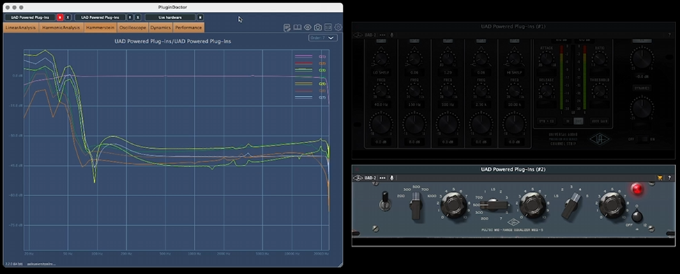
Remember that Precision Channel Strip equalizer plugin we discussed earlier? Let’s compare that to this Universal Audio Pultec MEQ-5 emulation. On the linear analysis, we can match up the frequency response of each plugin by adjusting the gain, frequency, and Q settings. So far, they look identical. But let’s take a look at the harmonic analysis.
Even if we reset the settings on each EQ, we can see that harmonic frequencies are excited just by simply running the signal through the Pultec. And the balance of those harmonics changes as we drive the input of the Pultec harder, while we never see any audible harmonic distortion with the Precision Channel Strip EQ.
The Precision Channel Strip EQ remains linear, no matter what we do to the settings. It’s perfect for fine-tuned, surgical adjustments. But this data tells me the Pultec might be better for when I want to add some character to a signal.
These results are even more interesting if we represent the information in another way… Instead of just sending a sine wave to these plugins, what would happen if we sent in a broadband signal with energy across the frequency spectrum?
In the first video, we demonstrate the Hammerstein tab within Plugindoctor. It gives us an idea of the effects we can expect at the 1st, 2nd, 3rd, 4th, 5th, 6th, and 7th order harmonics at varying input frequencies. The harmonics are color-coded to the key in the top right corner.
In the video, you can see that the Precision Channel Strip only shows information at the first harmonic (the fundamental frequency). Adjusting the gain structure at any point won’t impact the harmonic content generated, because there isn’t any audible harmonic distortion associated with this very clean digital EQ.
Running this test on the Pultec MEQ-5 tells an entirely different story though. Again, we see harmonic content across the frequency spectrum before even adjusting the settings on the EQ. When we start adjusting the levels, we see various patterns of harmonic content arise.
Attack, Release, & Ratio
Getting back to compressors and limiters, it’s not just the harmonic character that varies between analog hardware and plugins. There were also some idiosyncrasies built into classic models like the Universal Audio 1176 and LA-2A.
The 1176, for example, is capable of extremely short attack times (down to about 20 microseconds!). That proposes a serious obstacle for making a plugin emulation of the 1176, because 20 microseconds is even shorter than the sample length at a 44.1 kHz sample rate. Therefore it’s a bit difficult to detect the amplitude of the signal and control the gain within that extremely short time period.

However, as can be seen in Part 2 of ‘What is “The Analog Sound” by this measurement, the UA plugin emulation (on the bottom) is nearly just as quick as the reissue analog model (on the top) and the original unit (in the middle).

In digital playback, we also have the ability to look much further ahead in time at audio before it reaches the input of the compressor, which is something that can’t be done to the same degree with analog equipment alone.
The program-dependent release of the 1176 is also iconic. This means that the time it takes the compressor to stop compressing after a quick transient will be different from the release time after compressing a more tonal signal.
The graph below shows this behavior in action. You can see a quick burst of signal, followed by a relatively short release on the left. And in the center, you can see that a longer burst of signal results in a markedly longer release time.

This has big implications on how the compressor will sound on a drum kit, compared to a bass DI, compared to a vocal. Typical digital compressors simply don’t have this sort of nuanced behavior. You need analog hardware or plugin emulations of analog hardware for that.
Frequency Dependency
Another important nuance of analog compression can be found in the equally iconic Universal Audio LA-2A. This also has a unique program-dependent release. But it also exhibits frequency-dependent compression threshold and ratio.

Look at this graph and notice that (a) the compression begins earlier for some frequencies and later for others, but the compression also (b) intensifies at different rates for each frequency as the signal goes further beyond the threshold.
This is just another example of the very unique and nuanced behavior of analog circuits compared to a simple digital algorithm that doesn’t account for these infinitely small details.
Again, you can see by comparing the two graphs above, that the developers at Universal Audio created plugin emulations of the LA-2A that exhibit insanely realistic behavior compared to the original hardware.
And for those of us who were born into this industry with such advanced analog emulations already on the market, I think it’s important to realize just how incredible it is that many of these nuances can be so accurately captured and packaged into a plugin.
What used to cost thousands of dollars for a single channel can now be applied to multiple channels at a fraction of the cost – which is mind-boggling if you really stop to think about it.
Limitations of Digital Audio
There is also something to be said about the unique sound of each individual 1176 installed in studios around the world. Each 1176 could be subject to slightly different construction, history, or environmental factors that may make it sound different than any other 1176. And this isn’t necessarily a bad thing either. Some engineers know their analog gear so well that they might choose one LA-2A over the other for a specific task even though they are the same exact model.
While analog distortion is simply a natural reaction to overdriving an analog circuit, digital emulations of analog distortion must be specifically programmed to sound like analog distortion. And that’s not a simple task. That’s why I invited Universal Audio to sponsor a series of videos and blogs, because they are among the very best at creating faithful emulations of analog gear. If you haven’t yet, you can check part 3 of ‘What is “The Analog Sound”’, to hear some of the demonstrations we discuss below.

Back in the early days of digital audio, most plugins just carried out a relatively simple mathematical task to achieve the desired function of, say, a compressor or an EQ. Don’t get me wrong – this was still incredible technology for the time, but these days plugins can be much more sophisticated.
You can expect different sound coloration when you run a signal through each Universal Audio plugin, because each one is designed to emulate a different circuit, with unique tube, tape, or transformer characteristics modeled after the real gear. Not only that, but you can expect a different sound depending on the input signal level going into the plugin, just as you would when using the real gear. Many UA plugins even have headroom screws or bias settings or tape types that can be used to experiment with the click of a button. Features like this give you access to the character of analog gear without the inconvenience – a workflow that is only possible with digital.
Digital isn’t completely free of its own drawbacks though. One of the important limitations in digital audio is aliasing. A digital audio system can only accurately sample frequencies up to the Nyquist limit, which is half the sample rate in a digital audio system. So in a 48 kHz sample rate session, no frequencies beyond 24 kHz can be properly sampled. That’s why the input of your interface contains low pass filtering, so that those ultra-high frequencies can be removed before being digitized.

When you distort a signal in the digital domain, the higher-frequency harmonics that are excited can very easily reach the Nyquist limit. And once they do, they will fold back down into the audible spectrum as aliasing. Unfortunately, these artifacts won’t necessarily stick to a musical, harmonic series that is pleasing to our ears.
In the video, you can listen to the aliasing that occurs when using the stock DAW distortion plugin on a sine wave… The sine wave alone looks like this on the spectrogram – a straight line from 20 Hz to 20 kHz with equal energy throughout. But when I distort the signal with this simple digital distortion plugin, the harmonics quickly exceed Nyquist and turn into very obvious aliasing.

In a true analog piece of equipment like the Universal Audio 1176, there’s no need to worry about aliasing because nothing is being sampled. The higher frequencies that arise with harmonic distortion in the outboard gear will simply be filtered out by the time they reach the input of your A-to-D converter.
Several more advanced plugins have a feature called oversampling that will use an internal sample rate that is much higher than the session sample rate, increasing the Nyquist limit. You can see below that the aliasing that occurs in this UA plugin will be attenuated rapidly before returning to the audible range, which makes the aliasing problem much less noticeable.

With more and more excessive distortion, there is just nothing that can be done to completely solve this problem, but oversampling certainly helps in most situations.
The final difference between analog and digital audio that I want to mention is latency. One example of where latency becomes a problem is when you’re monitoring the input audio signal in real time while performing.
Signals in an analog system travel at about 70 percent the speed of light, which to humans is effectively instantaneous at any practical distance. This means the sound from your vocal microphone will reach your ears in your headphones at the instant you sing into the microphone, which is how we are used to hearing ourselves.
This makes for a more comfortable experience for the performer, which is one of the most important elements of capturing a great performance.
With digital systems, there is always a bit of latency (or delay). This is especially true if you want to process the signal that is being monitored. In a typical interface and DAW setup, the signal would need to go into the interface, through the DAW and plugins, then back out of the interface to the headphones. This processing and transport all takes time, which can add up. Assuming your computer is capable of operating at a low buffer size, it’s unlikely that the performers will be able to detect the tiny delay. But setting a low buffer size often means that the session needs to have fewer active plugins.

This is one reason why many engineers will run the signal through an analog compressor and mixing console before splitting it to the DAW for recording and the performer’s headphones for monitoring. But few of us can afford a nice console and a rack of outboard analog gear!

Some audio interfaces have internal DSP that helps with this problem. The Universal Audio Apollo interfaces for example have internal processors that allow you to run these analog hardware emulations we have discussed in real time with very low latency. So, you can use advanced processing like compression, reverb, and EQ in your monitoring mix.

If your interface doesn’t have an internal DSP, another option would be to use the direct monitoring button that sends the input signal to the headphones without going through the DAW first. The problem here is that you will only hear the dry signal, unaffected by the plugins in your DAW session.
The built-in analog compressor within the Volt 276 that we talked about earlier can be used here to control dynamics for both the recording and the monitor mix. Because this is an analog compressor, it introduces no latency and the effect can be heard when using direct monitoring on the interface.
This reminds me – there’s another important reason why many engineers work with a compressor or EQ in the signal chain while recording…
In today’s digital world, we have the tendency to save all of the mixing for the end. This is especially true for those of us who were born in the digital age. Young engineers tend to have a “fix it in post” mentality, as if all problems in the sound should be fixed after the recording.
But there is a lot to be gained by making decisions earlier in the production process. If we can learn to sculpt the sound of our recordings from the beginning, we will have a clearer vision of the sound we are building, which will usually result in better results in the end.